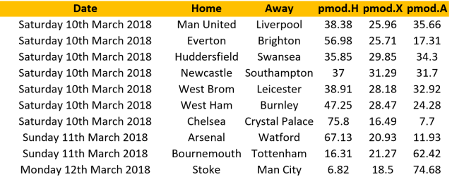

With 6 games played in the EPL, La Liga and Bundesliga it is now time to start running my PELICAN model again. The 3 tables below show the probabilities of home (pmod.H), draw (pmod.X) and away (pmod.A) outcomes for the week end fixtures. These can be used directly to look for value in the head 2 head markets or combined together if you prefer the so called “double chance”and “draw no bet” markets. Good luck and enjoy your football!


Over the last few weeks I have tried to document the different steps involved in building, tuning and testing a football prediction model (see here for episode 1). My aim was to provide the sort of basic concepts I would have liked to read about when I started with this hobby. Today’s article is the last one of this series and it is intended as a conclusion / where next wrap up.
In episode 5 we saw that the model we painfully built was most likely not going be profitable. However there were several reasons to be optimistic after this first attempt and the rather simple approach we implemented can now serve as a benchmark to beat (both in terms of the AUC metric and profitability). There are some obvious areas of potential improvement to focus on and here are just a few ideas:
So where to from here? Well first please get in touch if you end up building your own models, I am very keen to hear how that goes and happy to discuss any ideas. As far as the new season is concerned my plan is to post raw model probabilities on this blog each week (on Fridays), i.e. the Home / Draw / Away probabilities from the (upgraded) PELICAN model. I won’t put suggested value bets as I did in the past though as I want to keep the blog on the technical (rather than gambling) side.
But I do want to keep gambling… and document the experience as honestly as possible. For this reason we will be starting a new blog, and by “we” I mean my good friend Cyril (a.k.a. “squirrel”) and I. We will be using the PELICAN model to run a 10 000$ fund and the idea is to have the squirrel write about our ups and downs through the season. From experience I find it very hard to objectively assess how my model is doing so having someone else (with a much better sense of humour) judge PELICAN should be entertaining; and since the squirrel did put a lot of his own cash in the fund I trust him no to sugar coat his views…
Here is the link to this new blog: https://touchthesquirrel.wordpress.com/
We will post week end tips every Friday (so anyone can join the ride), quoting the odds we were able to grab and we will also review the fund performance monthly. Obviously there are no guarantees whatsoever on profit, except for the fact that we are backing every bets ourselves as reported.

Towards the end of my last article we settled on a model we thought performed well enough in terms of the AUC metric we introduced in episode 3. The model is a glmnet with input parameters set to alpha = 0.8 and lambda = 0.0019. The model predictions take the form of probabilities characterizing the likelihood of the home team winning. The aim of today’s article is to test these predictions against the betting market (finally…).
A first important aspect to understand is the concept of value betting: we won’t be using the model as a classifier, systematically betting on the most likely outcome (i.e. we don’t “tip” winners). Instead we want to identify games where the market price (here taken as the Bet365 odds reported by football-data.co.uk) looks too generous compared to our model’s assessment. Take as an example the Watford v Liverpool game on the opening day of the coming season. Bet365 currently have their odd for a Watford win set at 6. This means the implied probability is ~16.6% (1/6 ~ 0.166). Now imagine the probability estimate from our model for a Watford win (Home win) is higher, say 20%. This would translate into odds of 5 instead of 6 with the model hinting at the market being too generous (it pays a win at 6 where we believe it should only pay it at 5). In a case like this, and even though the model is clearly indicating there is a 80% chance that the game outcome will not be a home win, we will bet on the home team. To reiterate the idea, the model is not “tipping” a Watford win, it is only suggesting that if these teams were to play 5 games (in the exact same conditions) Watford would likely win one of them. Having that win paid at odds of 6 offers value and that’s what we are after.
This is called value betting and the logic is that if we consistently select bets where the market is too generous we will come out with a profit on the long run. Unfortunately that last bit is very important and this betting strategy might bring some very long losing runs before any profit can come in (see this this earlier post for a theoretical illustration).
Right, so we will bet when the model disagrees with the market and thinks it is too generous, but how much should we risk? It feels that if there is a 4 out of 5 chance that Watford will not win we should not bet too much (otherwise we could blow the bank before profits start to come in). One popular answer to this question comes from the Kelly formula, which I described in this earlier post. The key idea is that the portion of your bank to invest on a single bet depends on 2 things:
Applying the full amount that the formula predicts is very risky and usually not recommended in a situation like ours where we can only put limited trust in our model’s predictions (i.e. we don’t know the true probability of the event, only a modelled estimate). For that reason people usually bet only a fraction of the suggested amount (fractional Kelly).
Using the glmnet model as tuned in Episode 4 I have generated probabilities of a home win for every game in the testing dataset (i.e. season 2015-2016). Converting these to odds (1/prob), and after comparison to the Bet365 home odds, we can identify the games offering value: the ones where the model odds are lower than the bookies’. Note in this exercise we are only betting on home teams but the model can also be used in the same way to identify value bets on the draw/away “double chance” market.
I have then applied the Kelly formula assuming a Bank of 1000 units and a Kelly fraction of 1/8. The betting log for that exercise can be found in this file and the curve below shows how the bank would have evolved throughout the 15/16 season:
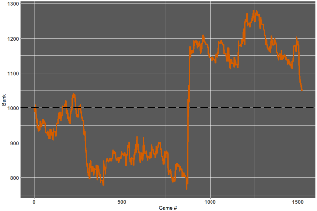
So we have a money making model? Well maybe on that season but the curve certainly hints at a very bumpy ride. The season was basically rescued by a single bet at very long odds (game # 874: Levante beating Atletico Madrid at odds of 17) and I would certainly not like to back a model like this too heavily.
How about last season which we left completely out of the entire analysis until now (see “validation set” in Episode 3)? We can rebuild our glmnet model now using a training set that goes all the way to the end of the 2015-2016 season. We then model the home win probabilities for the 2016-2017 season and apply the same betting strategy as above:
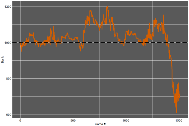
Yeah… we would have lost money on that one {see here for the betting log). Pretty disappointing after all this you might think? On the contrary I feel like these are pretty encouraging results given the simplicity of both the model and betting strategy. There are plenty of avenues for potential improvements, either by introducing new features, from an exploration of the other 200+ models available via the caret package, or by refining the conditions on when and how we bet.
In the next (and final) episode of this series I will discuss some of the steps that can help improve profitability, and will show how my model (PELICAN) performs on the various metrics we have seen so far.
In episode 3 we used our European football dataset to build some first predictive models. These were logistic regression models providing a probability estimate for a game ending either as a Home win (“H”) or not (i.e. draw or away win, which we labelled “X2”). We then assessed model performance in terms of the Area Under the Curve (AUC) metric when analysing ROC curves. The best we could achieve was AUC = 0.69 after applying some pre-processing to the data. In today’s article we will see how the caret package in R can help us test and tune other models to improve on this performance.
As stated in the package documentation caret is designed to “streamline the process of creating predictive models” and that’s exactly what we need here. In particular it allows to test over 200 models without the need to know their specific syntax or the details of their implementations. Some excellent examples of use (and the reason I started using the package) can be found in these 2 articles from Tony Corke (@matterofstats):
In this post however we will only focus on a single algorithm to describe how caret works. It should then be fairly straight forward to extend the work to other algorithms from the caret list (as is done by Tony in both articles listed above).
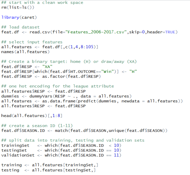
First let’s set up the framework and define our input features, target and the training/testing sets:
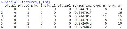
You will notice that there are a few extra steps compared to the setup we had in my previous post. First we are grabbing two more fields to be considered as input features: the leagues in which the game is being played (Div) and the season increment (SEASON.INC) both introduced in the first article of the series. Now a potential issue for many models is that the league indicator is a categorical input. The lines of code under the “one hot encoding” comment deal with this by converting the Div feature into 5 different binary fields. For instance the first 5 games listed below are all played in the premier league so have their Div.E0 field set to 1 and the others to 0.
The algorithm we will be using as example of the caret framework is called “glmnet” and belongs to the family of penalized logistic regression models. It is a natural extension to the glm model we saw in episode 3 but it now involves two tuning parameters that control the amount of “regularization” involved. I will not describe the algorithm but please have a look here or here if interested. Instead we will simply accept that this algorithm has two input parameters that can be adjusted to optimize the model performance (tuning parameters). This is where caret becomes very handy as it provides a single framework that works with any of the > 200 models available.
Similarly to what we did by splitting our data into training and testing sets, caret will allow models to repeatedly be built using a subset of the training data while the remaining data (holdout sample) is used to evaluate model performance. This is called resampling and several techniques exist (e.g. k-fold cross validation, bootstrapping etc…). In what follows we will use a 10-fold cross validation approach (see https://www.cs.cmu.edu/~schneide/tut5/node42.html). Essentially we randomly partition the data in 10 sub-groups of similar size, use 9 of them to build a model, evaluate its performance on the 10th (holdout) set and repeat. These 10 holdout estimates of model performance are used to understand the influence of each input parameter.
The following lines of code will set up our tuning run with caret:
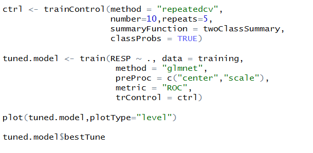
First we store information on how we want the resampling to be done (ctrl) and here we specify a repeated cross validation method (method = “repeatedcv”) with 10 folds and 5 repeats. As part of the ctrl definition we also indicate we will be using one of caret default summary function (“twoClassSummary”) to compute the AUC for a binary classification problem and that we are working with class probability predictions (ClassProbs = TRUE).
The call to the “train” function on the following line is how caret builds and tunes models. As for the glm model in episode 2 the first line indicates that our target is the field called RESP in the training dataset and that we want to use all other fields in that data frame as predictors. The attribute “method” is where caret is told which of the 200+ models to use (here glmnet). In this example we also tell caret how to pre-process the predictors (PreProc = c(“center”,”scale”)) and which performance metric to optimize (ROC).
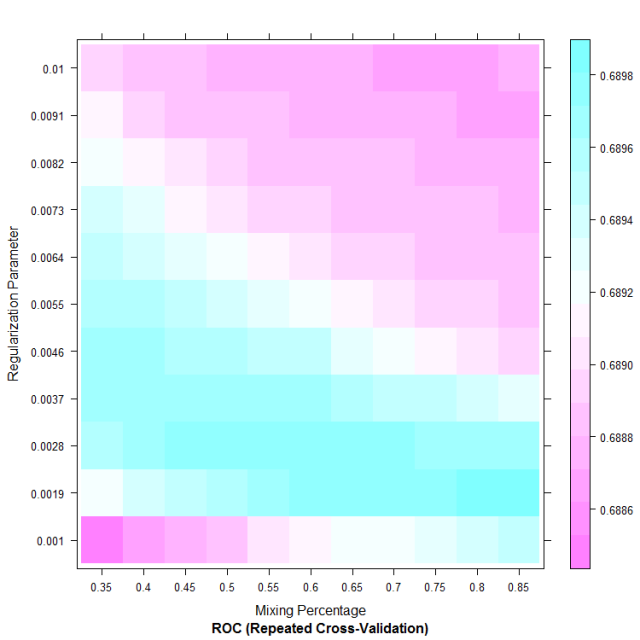
Without any further input information caret will then decide on a set of input values to test for each parameter in the model. This means you can test any of the 200+ models available using the same syntax as above without even knowing the names or number of input parameters required. From analysis of the holdout performance caret will identify the combination of input values that achieves the highest performance. The figure below summarizes the holdout performance for the default input values selected by caret for method = “glmnet”.
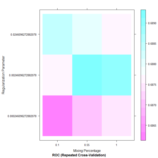
In this case the best holdout performance was achieved using alpha = 0.55 (mixing percentage, x-axis) and lambda ~ 0.0025 (Regularization parameter, y-axis). It is that setting that is used by default when making prediction with the tuned.model object where the results of the train call are stored (note the model is stored under tuned.model$finalModel). We can therefore check the AUC this model now achieves on the testing set by making predictions in a similar fashion to what we did in episode 3:
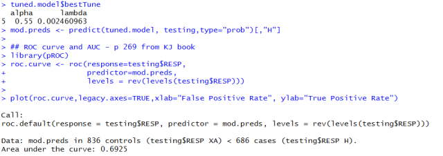
I won’t show the ROC curve but the AUC now reaches 0.6925 which is an improvement on what we had in Episode 3 (0.69).
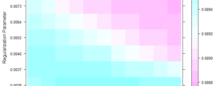
Can we perhaps get an even greater improvement by choosing better parameter values? Notice that the range of values selected for alpha and lambda by default was pretty broad (coarse grid resolution) and there might be a more performant combination around alpha = 0.55 and lambda = 0.0025. Caret allows you to specify the grid of values you want the model to be optimized on:
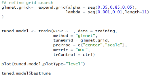
The best setting is now identified as alpha = 0.8 and lambda = 0.0019 (bottom right of the plot). However when checking the AUC for this setting on the testing set we still get a 0.6925 performance (no improvement). As a consequence we have probably reached the limit of what we can achieve with that particular model and there is little chance that further grid refinement will bring anymore improvement on the testing set: it is now time to check if that model can compete with the bookies!
In my next article we will review briefly how to set up a staking plan and will then have a look at how profitable (or not) this model would have been on the 2015/2016 and 2016/2017 seasons.
PS: one of the strength of the glmnet approach worth mentioning here is that it automatically performs its own feature selection (see episode 2). The following command shows which of the input features have been knocked out in the process (i.e. the one with no coefficient assigned). Note I am only showing the first 32 of the list:
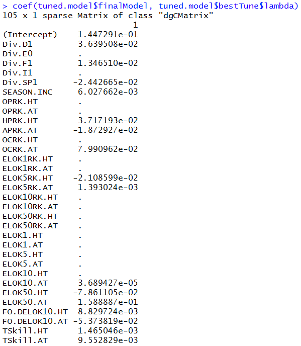
In the first post of this series we defined a bunch of variables (input features) that we thought might have some predictive power in determining the outcome of a football game. In a second post we then had a closer look at these features and got a feel for the ones that are likely to matter more. It is now time to use this data and build our first predictive models.
I already briefly mentioned the difference between a regression and a classification model and today the focus is on classification. Although there are technically 3 possible outcomes in a football games (home win / draw / away win) we will reduce this to a binary classification problem for now: a game either ends with the home team winning (which we will label “H”) or not (i.e. draw or away win, labelled as “XA”).
The following lines of code will format our dataset under this convention. I am also loading the package caret as it will be our main tool from now on.
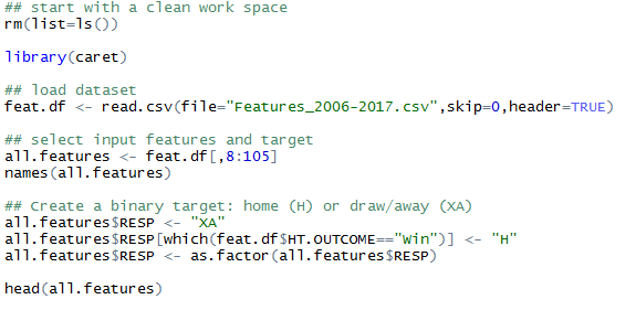
The aim of today’s article is to build a model that estimates the probability of the home team winning. As I mentioned in my last article we (usually) don’t want to use all our data when building a model. Instead the common practice is to leave aside a portion of the dataset for testing. As the model does not see that portion of the data during its training phase there is no risk that it might have somehow “memorized” the results (risk of overfitting). By making predictions on the left-out portion we can objectively judge the model performance. For this article we will be using the data from the 2006-2007 season up to the 2014-2015 one for model training. We will then test its performance on the 2015-2016 season (unseen during training). The 2016-2017 season is intentionally left out altogether and we will only use it as a very last check once we have settled on a “final” model in later posts (this is called the validation set). The following lines of codes should take care of the split:

Everything is basically set as if we were building a model in August 2015 using data from the past 9 seasons and we were about to start using it through the 2015-2016 season (remember the weird one with Leicester and all…).
There is a very large number of models available in this field but to lay down our modelling framework and get a benchmark on the sort of performance we can achieve I will start with an old, tested and trusted classic: logistic regression. If you want some details on the method this seems like a good place to go. I should also mention that most of what follows (today and in later articles) is based on the book “Applied Predictive Modeling” by Max Kuhn, author of the R package caret and p 282 has a good section on logistic regression. As I’ll be referring to that book you might want to consider investing in it (http://appliedpredictivemodeling.com/). However I also seem to remember finding a pdf copy for free somewhere online (but can’t find the link anymore).
Now let’s build this first model:
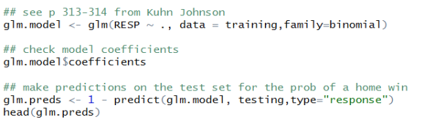
To check that nothing has gone too wrong we can have a look at the first 10 games where predictions were made:
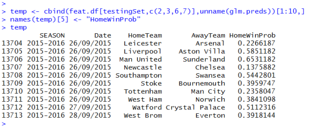
Right, so we have a model and it can predict stuff that sort of looks reasonable. Surely that’s not enough to go and start taking on the bookies though? No, and we do need to somehow assess how “good” these probabilities are.
For binary classification problems like this one the common approach is to check what is called a Receiver Operator Characteristic (ROC) curve. For an example of use in the context of Expected Goals models you might want to have a read of this recent article by @GarryGelade.
For our purpose the “event” we observe is a home win and the probability predictions can be seen as the level of confidence the model has that the event will occur for a given game. If we want a binary event / non-event prediction (H/ XA) we can choose an arbitrary threshold for the cutoff. This threshold can (for instance) be 50%, in which case a game will be predicted as a home win if the predicted probability is > 0.5. But maybe we want to be a bit on the safe side and take a buffer, say we will only predict a home win if the model has at least a 60% probability attached to the prediction?
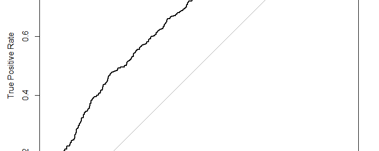
The ROC curve is a plot of the True Positive Rate (TPR: percentage of predicted home wins that are home wins; y-axis) as a function of the False Positive Rate (FPR: percentage of draw/away wins that are predicted as home wins; x-axis) for a range of thresholds between ~100% (left of the plot) and ~0 % (right of the plot).
TPR = # home wins predicted as home wins / # home wins
FPR = # XA predicted as home wins / # XA
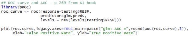
The following lines of code will provide the ROC curve for the test set:
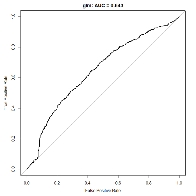
If we start at the bottom left of the plot the threshold selected to distinguish events (home wins) from non-events are very high: we only predict a game to be a home win if the model has very high confidence. For a good model we should therefore expect a large portion of these games to be home wins (high TPR, low FPR). This is however not the case at all for our model, and the bottom left of the plot has basically TPR = FPR (ROC curve following the 1:1 line) which means no skill at all – this model is easily fooled when it is highly confident! Things however get better as we lower the threshold (moving towards the right of the plot) and TPR becomes larger than FPR (ROC curve above the 1:1 line).
The common metric to summarize a ROC curve is the Area Under the Curve (AUC) which measures the area between the 1:1 line and the ROC curve. In this case the AUC is 0.643 and the goal from now on will be to increase its value.
The other thing people tend to look at is the probability calibration. Basically how often do we observe a home team winning in games where the model assigns a home win probability of 0.5? 0.2? 0.9? If the model probabilities are well calibrated then they must reflect the true likelihood of the event and, over a large sample set, we should see ~50% of games assigned a 0.5 probability end as a home win.
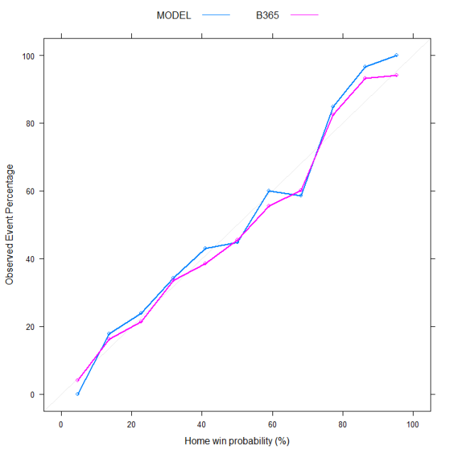
The code below generates what is called a calibration plot on the test set. The model predicted probabilities for a home win are on the x-axis and their frequency of occurrence (observed) is on the y-axis.
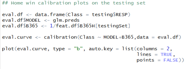
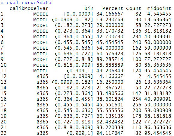
You can see (line 3) that I am also using the B365 home odds to obtain a probability that reflects the market’s point of view (prob = 1/odd). The calibration plot for the 2015-2016 season is shown below:
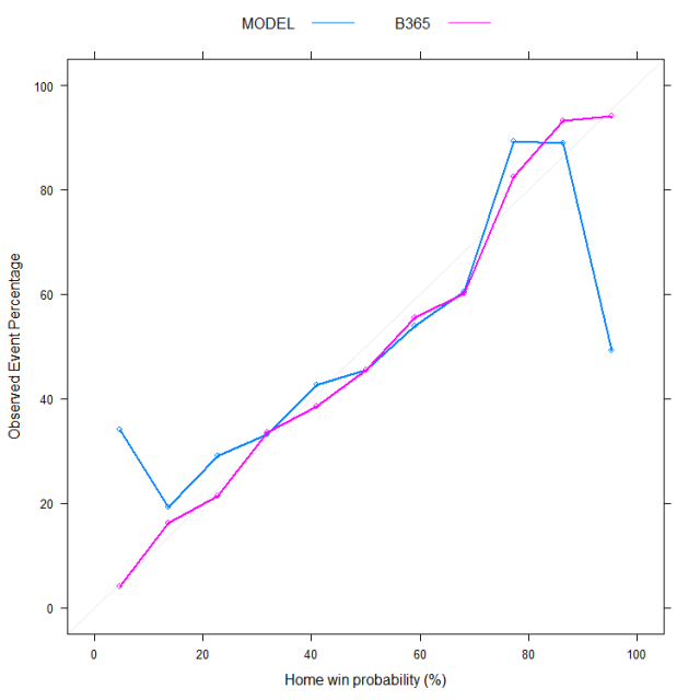
For probability estimates between ~ 10 – 90% the model seems to behave reasonably with observed outcome frequencies in the same ball park as what the probabilities imply. Arguably the market predictions are better (they are closer to the 1:1 line) but the model is not too far off. For the more extreme probabilities however (e.g. <10% or > 90%) we get the same problem as with the ROC analysis: the model is way too confident in its predictions. As the data below shows, only 49.2% of those games where the model assigns a probability of home win > 91% actually end up with a home win (last blue point on the right) while over 34% of games assigned a probability < 9% do end up as a home win.
Conclusion? Well if we really had to use this model we would need to discard predictions where the probabilities are >90% or <10%. Luckily we don’t have to use this model and we still have plenty of ways to refine our approach.
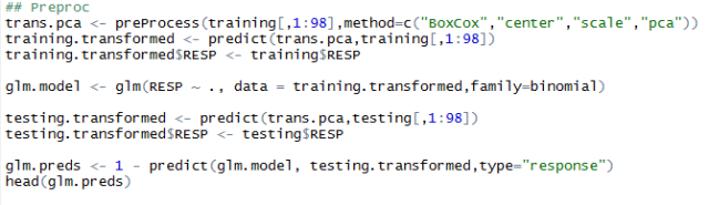
Before we start to explore and tune more complicated models (next post) I want to show a way to improve this simple glm with some pre-processing of the inputs.
I won’t go into the details of the pre-processing steps here as it feels like this post has gone for long enough already. Chapter 3 of the “Applied Predictive Modeling” book describes key pre-processing techniques such as the ones used below. To get some overview of what Principal Component Analysis (PCA) is you can also have a look at this earlier post. As discussed in the post a lot of the variables we use here are highly correlated (think shots and shots on target for instance) and PCA offers a way to deal with highly correlated features.
The code below will take care of the pre-processing thanks to caret and the updated ROC and calibration curves are also shown. Note that both the training and the testing sets need to be transformed in the same way.
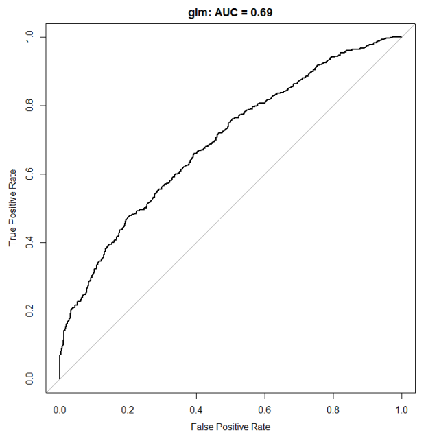
Much better, no? The calibration curve now follows more closely the 1:1 line, especially for the more extreme probabilities and our AUC has now jumped to 0.69. In my next post we will see if we can further improve this AUC performance using (and tuning) more complex models. We will also start to look at their performance in terms of betting returns because, well, at the end of the day this is what we are really interested in.
If anyone wants to start looking into betting returns from this glm-pca model I have put enough info in that file so that it can be done… I must admit though that I don’t have much hope that this model would be profitable at that stage.
In the first post of this model building series we introduced a dataset of ~ 100 features. These were chosen because of their potential to provide some information on the outcome of a future football match (predictive skill). In today’s post we will explore how important these features are (if at all) using the random forest algorithm. The exercise will also allow ranking of all features in terms of their predictive skill. From analysis of the most highly ranked parameters’ values we can hope to quickly judge a team’s strength at any point in the season and compare it to other teams, from current or previous seasons. More importantly we will get a feel for which features are critical and which can potentially be omitted when we build our predictive models. The results are however just indicative and by no means a definite answer: a feature labelled as “unimportant” might still be helpful in some cases and improve the performance of some models.
The set up
Although we will revisit these notions in more details in my next article there is a need here to introduce some modelling terminology as we are about to build our first models.
Input features (or predictors): the fields on which our model predictions will be based (see first post). In today’s example we will use all fields from column 8 to 105 from our dataset.
Target: what we are actually trying to predict. As we want to estimate game outcome and teams’ strength I will be using the game margin (from the point of view of the home team) as a target:
home team margin = home team goals – away team goals
As this is a numerical value rather than a categorical field the models we will build are referred to as regression models (as opposed to classification models).
Training data: the portion of the data from which the model will learn. It is usually only a subset of the full dataset (e.g. 70-80%) as the rest is kept for testing purpose. One of the particularities of random forests however is that it can be trained and tested on the same data (see below). This is the approach taken here and the full dataset will be used for training. Keep in mind however that this is very bad practice for most other algorithms and we will discuss why in the next article.
Methods: decision trees, random forests and the boruta package.
(If you are only interested in the results, skip this section)
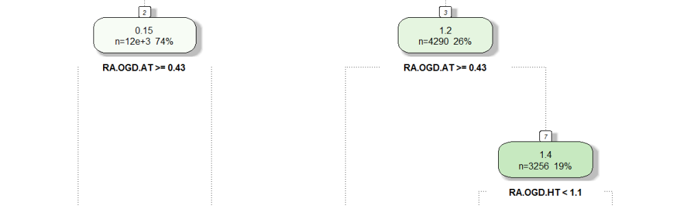
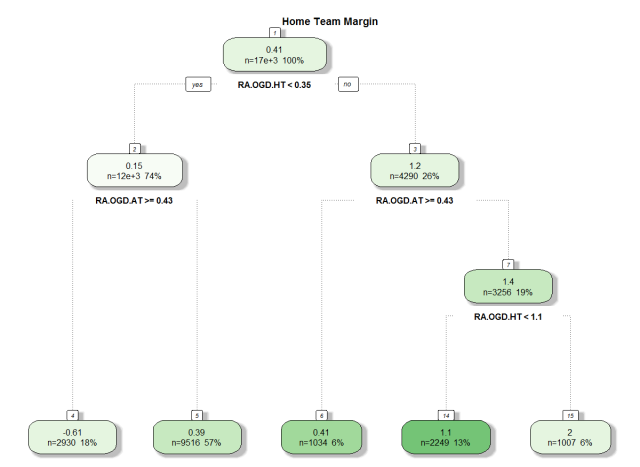
The building block to understanding what a random forest does is another algorithm called a decision tree. As shown below the goal of decision tree is to recursively partition the training data into smaller groups that are more homogenous with respect to the target. This is done via a series of nested if-then statements at the “nodes” of the tree, each time selecting a predictor variable to split the data and a threshold value for the split. The data in the terminal nodes (leaves) is then used to make predictions, for instance by taking the average of all target values in that subgroup. The figure below shows a very simple decision tree targeting the game margin from knowledge of the season-to-date average goal difference per game for each team.
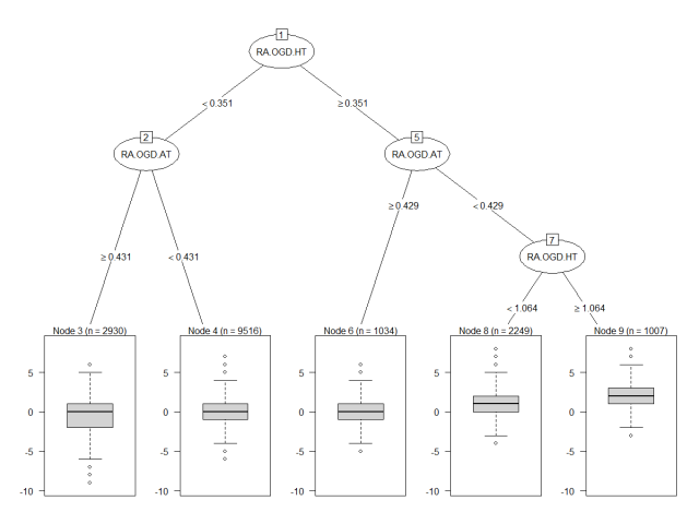
The data points in node 3 (bottom left) correspond to games in which the home team had a season-to-date average goal difference per game below 0.35 (left at node 1) and the away team had theirs above 0.43 (left at node 2). The distribution of the 2930 games that match these criteria is summarized by the box plot and you can see how it contrasts with that of node 9 for instance (bottom right) where the home team is a much clearer favourite. In many ways the only thing we have done here is to re-organize the data in groups that make sense in terms of game margins. How is that a prediction model? well when a new game is about to kick off you can look at the season-to-date average goal difference per game for each team, go down the tree and base your prediction on the data in the terminal node you end up in. The common way to do that is simply to take the mean of the data in the terminal node, as shown below. There are however other alternatives, such as building a regression model with the node data points.
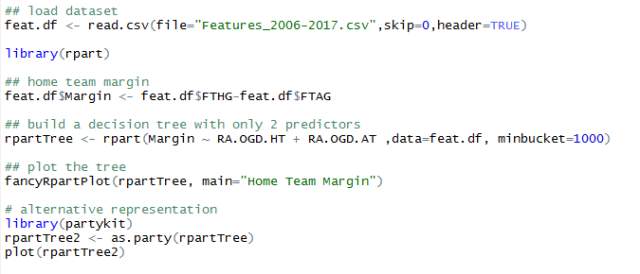
This was a very simple example with only 2 predictors and the R code I used is shown below. It can easily be changed to account for more predictors in the rpart call (line 7).
if you are new to R this might be worth a read.
Decision trees are easily interpretable and that’s why they are very popular as explanatory models. However they are also known to lack stability and small perturbations in the data can easily lead to very different tree architectures and/or splitting criteria. The accuracy of the predictions they produce is also easily outperformed by other (less interpretable) algorithms.
That’s where random forests come in. They help overcome these issues by combining a large number of decision trees (an ensemble) under the following conditions:
(1) each tree in the ensemble is given only a portion of the training data (called a bagged version, i.e. a random subset of the data sampled with replacement).
(2) only a random subset of all input features are evaluated at each node in the trees.
The final prediction from the forest is then obtained by averaging the predictions from each tree, improving both model stability and performance.
The other major strength of the random forest approach in the context of what we are trying to do today is that a portion of the data is left out when training each tree in the ensemble; these “out-of-bag” samples can be used to evaluate tree performance during the training process. In other words the entire dataset can be used for both model training and evaluation simultaneously. To obtain a picture of the importance of a given predictor, the algorithm can record the reduction in performance that results from a random shuffle of that predictor’s values across the training records. An importance estimate can then be assessed from the mean reduction in prediction performance (compared to that obtained with the original predictor) on the out-of-bag samples and averaged over all trees that use that predictor. This allows ranking of all input features in terms of their importance.
The Boruta package is built for this purpose: it is a wrapper around the random forest algorithm and allows identification of features that are not relevant by comparing their importance score to some “shadow features”. These shadow features are random and their importance scores are therefore only attributable to random fluctuations. Any input feature that does not register an importance score significantly higher than the maximum score from the shadow features is considered unimportant and can (maybe) be omitted from the set of inputs.
Results
To rank our input features in order of importance using Boruta I have essentially followed that post.
The code I used is shown at the end of the article, however be aware that it runs very slowly due to the size of the dataset. If you want to run it yourself I recommend using only a portion of the data (maybe the last 4 seasons only) and/or a subset of all features. If you have the patience you can run the full dataset and hopefully results should be similar to this:
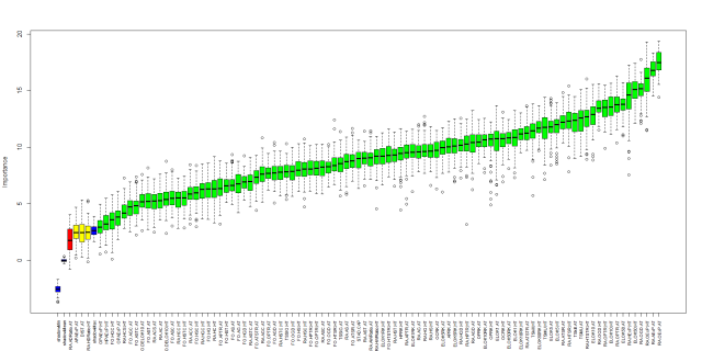
which in table form gives you the following ranking:
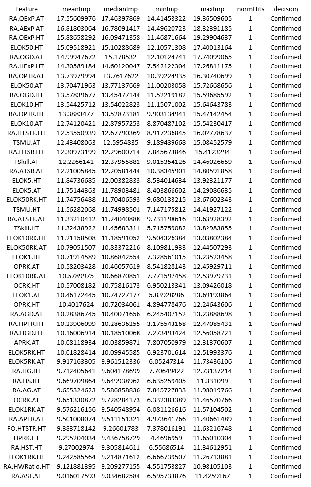
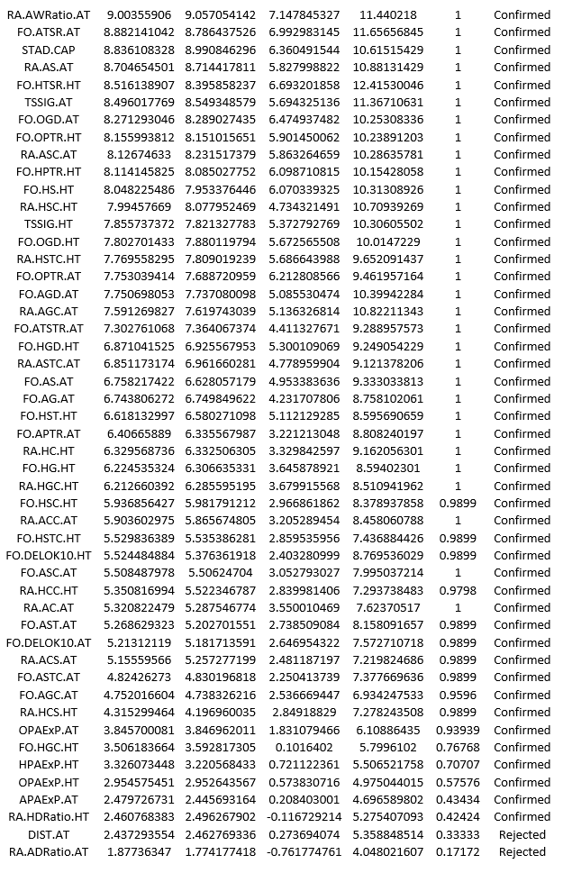
As far as predicting game margins goes the top 3 most important features are linked to market expectations on the average number of points per game each team should have collected in the season-to-date. Perhaps this was to be expected as to some extent these metrics account for the info in the other features. After that we have the ELO ranking for the home team with a weight of K=50 in 4th place while the average goal difference per game for the away team comes in 5th. The total shots and shots on target ratios running averages (RA.TSR and RA.TSTR) are all ranked in the top 25 indicating they are perhaps the best way to look at shot statistics (as has been argued by many on twitter). The first form indicator (FO.HTSTR.HT) only appears at the 44th position with most of the other metrics from that family well into the second half of the ranking. This also confirms what many have found about the danger of reading too much into recent results when trying to assess future performance.
At the other end of this ranking we find the “points above expectation” (PAExP) metrics, the two features based on teams’ draw ratios as well as the distance travelled. Now I could easily be convinced to drop the draw ratio indicators as well as the PAExP ones as they surely have a huge random component. However I’d like to see more evidence that the distance travelled is not useful before to give up on it…. and that’s where the fiddling starts! In the third post we will define a framework for model evaluation and iteratively add/remove some of the features, recording the change in model performance along the way. This will also produce our first predictive models that can be tested against the market in terms of profit/loss over an entire betting season.
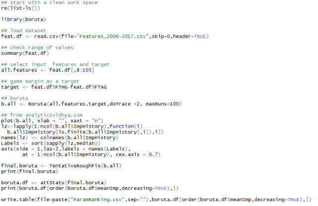
Code for the Boruta rankings (after https://www.analyticsvidhya.com/blog/2016/03/select-important-variables-boruta-package/)

Here we are with the first post of this model building series. I suppose if we really wanted to be thorough there should be a “Step 0: data scraping” post but the truth is we are fortunate enough to have the work of Joseph Buchdahl (@12Xpert) at football-data.co.uk. The data he provides here is the starting point for most of what I have done. I am also grateful to Jonas (@opisthokonta) for his stadium coordinates dataset available here. So let’s go past Step 0 and dive straight into what I personally find the most frustrating task: feature engineering.
The idea here is to derive all the metrics we think might have some predictive skills, and the reason I find it so frustrating is that it NEVER ends. There is this constant doubt that you can add something else that might greatly improve model performance, be it the weather, the distance players have to travel or any of a thousand ways of judging a team’s strength. The other aspect I find very frustrating is that there are no obvious ways to decide on the best subset of features to use – yes some algorithms do give you an idea of feature importance (and we will discuss this in the second post of the series) but at the end the whole exercise is more of an art form than a clear procedure. From what I have seen what you end up using or not is down to your experience, taste and a whole lot of trial and error (i.e. model evaluation).
In many ways this is the task that has taken me the most effort and I realize that not having a decent set of features is a bit of a barrier to entry to anyone wanting to have fun building models. For this reason I have uploaded a dataset of features here which covers games in the 5 major European leagues since 2006 (16735 games). The problem is that for it to be useful I need to somehow explain my poor notation… there are ~100 features in that dataset so the task is a bit tricky! The rest of the post will introduce the metrics and notation used so bear with me a little longer if you can, otherwise just grab the data and have “fun”.
Dataset link: https://www.dropbox.com/s/r9c8sehvccgyxtn/Features_2006-2017.csv?dl=0https://www.dropbox.com/s/r9c8sehvccgyxtn/Features_2006-2017.csv?dl=0
Overview of metrics and concepts
Let’s start from the beginning: the football-data.co.uk dataset. The definition of fields in that dataset is available here and it covers both results and game statistics.
The first thing to understand is that we are building a predictive model, and can therefore only use information on a team’s past performance. When trying to estimate the probability of Team A winning game X we can use all information about Team A and its opponent that was available prior to kick-off, but only that. Using the number of shots taken by Team A in game X would be wrong as this information was not available before kick-off. For any given game we therefore want to get an overview of teams’ performances prior to the game. For this I use 2 families of features:
Examples of metrics that get averaged like this include goals scored (conceded), shots (on target) scored (conceded) etc…
Now looking at shot statistics is not the only way to evaluate a team’s performance. Among the many different rating options I have used the following:
The remaining of the post is simply a README for the dataset and at that stage I really recommend just downloading the file and staring at it while going down the list below. In my next post we will start playing with that dataset in R on our way to building a predictive model.
FEATURE LIST
Game info
Div: League Division as defined by football-data.co.uk
SEASON: label for the season
Date: DD/MM/YYYY
SEASON.INC: increment (0 to 1) indicating how late in the season the game is played.
Game.id: identification number for the game
HomeTeam: home team
AwayTeam: away team
Model features:
OPRK.HT (OPRK.AT): Previous season final table position for the home (away) team.
HPRK.HT (APRK.AT): Previous season final table position for the home (away) team when only accounting for home (away) games.
OCRK.HT (OCRK.AT): Current table position for the home (away) team
ELOK1RK.HT (ELOK1RK.AT): ELO ranking using a weight factor K=1 for the home (away) team
ELOK5RK.HT (ELOK5RK.AT): ELO ranking using a weight factor K=5 for the home (away) team
ELOK10RK.HT (ELOK10RK.AT): ELO ranking using a weight factor K=10 for the home (away) team
ELOK50RK.HT (ELOK50RK.AT): ELO ranking using a weight factor K=50 for the home (away) team
ELOK1.HT (ELOK1.AT): ELO ratings using a weight factor K=1 for the home (away) team
ELOK5.HT (ELOK5.AT): ELO ratings using a weight factor K=5 for the home (away) team
ELOK10.HT (ELOK10.AT): ELO ratings using a weight factor K=10 for the home (away) team
ELOK50.HT (ELOK50.AT): ELO ratings using a weight factor K=50 for the home (away) team
FO.DELOK10.HT (FO.DELOK10.AT): change in the home (away) team’s ELO rating (K=10) in the last 4 games.
TSkill.HT (TSkill.AT): TrueSkill ratings for the home (away) team
TSMU.HT (TSMU.AT): TrueSkill mu value for the home (away) team
TSSIG.HT (TSSIG.AT): TrueSkill sigma value for the home (away) team
STAD.CAP: stadium capacity (home team)
DIST.AT: distance travelled by the away team (using stdium coordinate dataset from opisthokonta.net)
RA.HS.HT (RA.AS.AT): Season-to-date average number of shots registered per game by the home (away) team when playing home (away).
RA.HST.HT (RA.AST.AT): Season-to-date average number of shots on target registered per game by the home (away) team when playing home (away).
RA.HSC.HT (RA.ASC.AT): Season-to-date average number of shots conceded per game by the home (away) team when playing home (away).
RA.HSTC.HT (RA.ASTC.AT): Season-to-date average number of shots on target conceded per game by the home (away) team when playing home (away).
RA.HG.HT (RA.AG.AT): Season-to-date average number of goals scored per game by the home (away) team when playing home (away).
RA.HGC.HT (RA.AGC.AT): Season-to-date average number of goals conceded per game by the home (away) team when playing home (away).
RA.HGD.HT (RA.AGD.AT): Season-to-date average goal difference per game for the home (away) team when playing home (away).
RA.OGD.HT (RA.OGD.AT): Overall (home and away games) season-to-date average goal difference per game for the home (away) team.
RA.HTSR.HT (RA.ATSR.AT): Season-to-date average TSR (total shot ratio) per game for the home (away) team when playing home (away).
RA.HTSTR.HT (RA.ATSTR.AT): Season-to-date average TSTR (total shots on target ratio) per game for the home (away) team when playing home (away).
RA.OExP.HT (RA.OExP.AT): Market expectation (using b365 odds) for the average number of points per game (home and away) for the home (away) team in the season to date.
RA.HExP.HT (RA.AExP.AT): Market expectation (using b365 odds) for the average number of points per home (away) game for the home (away) team in the season to date.
RA.HC.HT (RA.AC.AT): Season-to-date average number of corners per game for the home (away) team when playing home (away).
RA.HCC.HT (RA.ACC.AT): Season-to-date average number of corners conceded per game by the home (away) team when playing home (away).
RA.OPTR.HT (RA.OPTR.AT): Season-to-date average ratio of points gained to max points possible per game for the home (away) team. 3 points for a win, 1 point for a draw.
RA.HPTR.HT (RA.APTR.AT): Season-to-date average ratio of points gained to max points possible per home (away) game for the home (away) team.
RA.HWRatio.HT (RA.AWRatio.AT): Season-to-date average ratio of home (away) games won by the home (away) team.
RA.HDRatio.HT (RA.ADRatio.AT): Season-to-date average ratio of home (away) games drawn by the home (away) team.
RA.HCS.HT (RA.ACS.AT): Season-to-date average number of Clean Sheets for the home (away) team when playing home (away).
All other variables starting with “FO.” instead of “RA.” Are a repeat of the above but averaging over the past 3 (home/away) games only and 4 games for overall (home & away) stats.
OPAExP.HT (OPAExP.AT): Overall points above market expectation (using b365 odds) for the home (away) team in previous season.
HPAExP.HT (APAExP.AT): Points above market expectation (using b365 odds) for the home (away) team in all home (away) games from previous season.
Model targets
HT.OUTCOME: match results from the point of view of the home team (Win, Draw, Lose). This relates to the 1X2 head to head market.
TOTALG.OUTCOME: is the match ending with less than 3 goals (under) or not (over). This relates to the over/under 2.5 goal market
Game outcome (not to be used for modelling)
These are taken straight from football-data.co.uk
FTHG = Full Time Home Team Goals
FTAG = Full Time Away Team Goals
FTR = Full Time Result (H=Home Win, D=Draw, A=Away Win)
HTHG = Half Time Home Team Goals
HTAG = Half Time Away Team Goals
HTR = Half Time Result (H=Home Win, D=Draw, A=Away Win)
Market odds from 3 mainstream bookies
from football-data.co.uk
B365H = Bet365 home win odds
LBH: Ladbrokes home win odds
WHH: William Hill home win odds
B365D = Bet365 draw odds
LBD: Ladbrokes draw odds
WHD: William Hill draw odds
B365A = Bet365 away win odds
LBA: Ladbrokes away win oddsWHA: William Hill away win odds

After a bit of a gap year in my blogging activity I am keen to get back to the sort of things I was doing during the 15/16 season – exploring machine learning techniques that might help us identify value bets. Since we have a month before the new season starts, and because my models have evolved considerably last season, I thought I’d go through the basics again.
In the next few weeks I will post a series of articles reviewing how to build a model that predicts the probability of winning, drawing or losing for a given team. My aim this time round is to give enough information (and data) for a keen reader to build a model that competes with mine… so sharpen your R skills and stay tuned!
I will then write a refresher on how such a model can be used to identify potential value in the market and we will go through how to set a staking plan again. Most of this info however is already on the blog and I don’t plan to change much for the coming season.
 Finally we will start betting again! I will be posting model probability estimates each week, starting in October (after the model has warmed up) for the 5 major European leagues (England, Spain, Germany, Italy and France). I will also provide these estimates to Alex (@fussbALEXperte) weekly for his model comparison project. Oh and a big thank you for the art work Alex!
The first post will be on feature engineering and we will look at what might be good predictors of a game outcome. The idea is to refresh this with the work I have done last year. Hopefully coming very soon…
I have not written much on here since the start of the 16/17 season but we have now gone through 12 rounds in the EPL and I suspect this is enough to start playing with the model again!
Recently I have been arguing on Medium that we should really aim to quantify as much as possible when making predictions and this is the angle I took when assessing each team’s likely finishing position.
I have written a much more extensive article on Medium about how I got to these results and here I want to jump straight to the results:
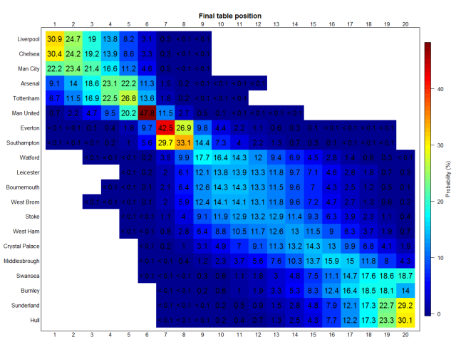
Liverpool and Chelsea are currently leading the pack with a 30-31% chance of being Champions while Man City is also in the mix with a 22.2% chance. Behind them a tight battle for the 4th Champion’s league spot could be on the cards for Arsenal and Spurs, and the model sees a clear top 8 that also includes Man United, Everton and Southampton. Among all teams/positions the highest probabilities identified are that of Man United ending 6th and Everton 7th. At the lower end the model sees Sunderland and Hull as the most likely to finish rock bottom while Burnley and Swansea should end up fighting to avoid the last relegation spot.
